
Understanding risk in its various forms is central to doing business and the PPA market is no exception in that regard. Discussions with many of our customers have shown that credit risk pricing for PPAs is an issue of concern for them which has not really been addressed for as of yet. This expertise gap prompted us to consider applicable methodology.
Credit risk is a crucial aspect in contract structuring for the renewable energy market. This article will explore credit risk and its various drivers in the context of the European PPA market.
Expected Loss and Credit Loss
First, the basics: Consider expected loss (EL), which is driven by three distinct factors:
- Probability of Default (PD) – ‘How likely is it that the counterparty may default?’
- Exposure at Default (EAD) – ‘How much is at stake should the counterparty default?’
- Loss Given Default (LGD) – ‘What fraction of the money at stake is actually lost?’
Credit loss materialises in the third stage, which is the culmination of the first stage (the default) and second stage (the level of exposure), with foreclosure and the liquidation / recovery process as the logical, if undesired outcome.
Probability of Default (PD): A Closer Look
The probability of default (PD) is driven by three factors:
- The financial strength of the counterparty;
- Some form of volatility, which determines how quickly financial strength might decline; and
- Transaction tenor. The longer it is, the higher the probability that default will occur at some point.
For very large corporates there are usually traded insurance-type contracts which benchmark default probability, the so-called credit default swap (CDS), which gained infamy during the 2008 financial / sub-prime mortgage crisis. However, such instruments are rarely written on utility firms in Europe.
Credit rating agencies such as Standard & Poor’s (S&P) and Moody’s gauge PD by assessing credit risk based on various qualitative and quantitative factors. These agencies rank the credit quality of debtors by assigning them to different rating classes, based on their financials, as for example tabulated below:
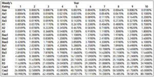
For each rating class, default rates are implied by stating the default probability up to different time horizons. A Monte Carlo simulation, allows for generating default time scenarios consistent with default tables.
Exposure at Default (EAD): A Closer Look
EAD is the amount of money at stake should a default occur. Depending on whether the payments are currently owed or will be owed in the future, there are two types of exposure:
- Settlement Risk Exposure (SR): How much has been delivered, but not yet paid for? SR is always defined by the exposure of the buyer towards the seller. Under standard EFET (European Federation of Energy Traders) terms, payments for electricity are due on the 20th of the month following delivery. A typically applied measure for SR, is the value of three monthly deliveries, based on the assumption of foreclosure being initiated after three months.
- Replacement Risk (RR): The differential between undelivered volumes valued market prices vs initially contracted prices. If and when default occurs, either the buyer or the seller can be exposed, depending on where prices have moved since deal closure. For the affected party, this is the loss that is incurred when entering into a replacement transaction at market rates.
RR is a little trickier to fully grasp than SR. Therefore, by way of example, consider the steps that a back-to-back energy trader needs to undertake after default has happened. We will analyse this from both the buyer’s and seller’s perspectives.
RR Example A : The Buyer is Exposed
In 2018, Bob bought power for delivery in 2023 from Alice at 40.00 EUR/MWh in order to sell it to Caroline. Today, the traded price for power to be delivered in 2023 is 45.00 EUR/MWh. Alice defaults today and will no longer be able to make agreed deliveries for 40.00 EUR/MWh in 2023.
However, Bob is still contractually obliged to deliver to Caroline and has to go to market to procure missing volumes at today’s price of 45.00 EUR/MWh. Bob as the buyer ends up paying 45.00 EUR/MWh for volumes which will be sold at 40.00 EUR/MWh to Caroline.
This equates to a replacement loss of 5.00 EUR/MWh.
RR Example B: The Seller is Exposed:
In 2018, Bob has bought power for delivery in 2023 from Alice at 40.00 EUR/MWh in order to sell it to Caroline. Today, the traded price for power to be delivered in 2023 is 35.00 EUR/MWh. Caroline defaults today and will no longer be able to take agreed deliveries at 40.00 EUR/MWh in 2023.
That means Bob is now left with surplus volumes, which he will no longer be able to sell to Caroline. He needs to liquidate the position by selling it in the market at 35.00 EUR/MWh, thus realising a replacement loss of 5.00 EUR/MWh.
There is more to consider with RR exposure, namely that it is dependent on two factors:
- Volume: RR refers only to non-delivered volumes, i.e. volumes still outstanding between the time of default and the contract end date. The volume subject to RR thus reduces with time.
- MTM: This is the difference between the contract price and the fair price of outstanding volumes. When the fair price of remaining volumes is lower than the contract price, the seller has RR exposure in the form of negative mark-to-market. A counterparty default would force them to enter into a replacement transaction at a lower price.
Thus RR exposure is driven by two counteracting factors: MTM uncertainty that increases with time and, conversely, volume (V) which decreases over time, giving the MTM trajectories the following shape:

The above graph shows 100 plotted simulations of the MTM for a 10y-year PPA over time. We have assumed that the PPA is closed at fair value, i.e. the MTM at the beginning of the simulation is zero. During an initial period of around, say, 2 years, the range of MTM realisations increases due to price volatility.
The progressive reduction of outstanding volume reduces the range of MTM realisations beyond this initial period.
EAD and Credit Risk
The relevance of EAD becomes clearer when one measures how much RR exposure might build up in the future. The essential drivers of EAD within the context of RR considerations are two-fold:
- Market volatility: The higher it is, the larger price moves will be, thus creating RR exposure
- Time: The more time passes since transaction closure, the larger uncertainty on future market price. Delivery counteracts this effect, whereby as delivery reduces outstanding volume, so the size of yet-to-be-delivered volumes shrinks, thereby reducing potential exposure.
It’s worth noting that credit simulations are joint simulations of MTM exposure and default. If and when default occurs in a simulation scenario, the EAD of the scenario is used to determine the amount lost. Pexapark employs these simulations to determine the distribution of potential losses.
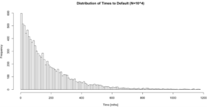
The figure below shows the distribution of 10,000 default times simulated for a counterparty with a low credit rating (Baa3):
After simulating default times and MTM trajectories, both need to be combined in order to calculate loss events. Determining whether or not a loss occurs after default is done via the following logic:
Scenario A:
Default time > tenor of the deal: In this instance, the offtaker has not defaulted during the contractual period of the PPA, therefore no credit loss occurs. All good!
Scenario B:
Default time <= tenor of the deal: In this instance, the offtaker defaults during the contractual period of the PPA. There are two possible sides to this occurrence:
1. If the MTM is positive, then the seller is not exposed, and the offtaker’s default does not lead to financial loss. On the other hand…
2. If the MTM is negative, then the seller is exposed, and the offtaker’s default will result in loss.
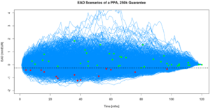
The simulation is conducted for a large ensemble of scenarios, leading to a set of credit loss realisations. Below is a combination of default and EAD simulations:
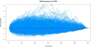
The diagram above shows 1000 plotted simulations of EAD over time.
For each EAD trajectory where default occurs, a point marks the time of occurrence. If the mark-to-market at default is negative (i.e. below the dashed zero line), a loss is realised (red points). Conversely, if it is positive, then no loss occurs (green points). It is on this basis that loss probability distributions can be computed.
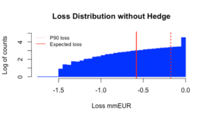
The histogram below shows the distribution of credit loss amounts contingent on default occurring:
The Mitigation of Credit Risk
Risk management is all about the limitation or mitigation thereof. There are various ways in which credit risk in the PPA market can be mitigated. These include:
- Contractual mechanisms: Advance payments, MACs (material adverse clauses), increased payment frequency, etc.
- 3rd party credit enhancements: Credit insurance (e.g. GIEK in Norway, SID Bank in Slovenia, etc.), Letters of Credit (LoCs), Parent company guarantees (PCGs). Credit enhancements cover exposure to the extent that the guarantor’s creditworthiness replaces that of the counterparty. Losses on the ensured/guaranteed amount will only occur in the event of double default of both the counterparty and guarantor.
- Collateral: Besides LoCs, counterparties may exchange other forms of collateral (cash, liquid securities) on an escrow account. In the event of default, the affected party is entitled to liquidate the collateral in order to indemnify itself against losses incurred.
- Traded credit risk: These are in the form of the aforementioned CDSs, as well as credit options or corporate bonds.
Simulating the Impact of a Credit Hedge
So, how does Pexapark assess a given credit risk mitigation measure in terms of loss distributions? The two plotted graphs below demonstrate this, with both plots having an identical set of EAD/default simulations.
The first figure illustrates a PPA deal with no credit protection applied, i.e. the line that divides the zero loss region from the loss region is at EAD=0:

The second figure shows a PPA deal with a guarantee to the amount of 250 kEUR, i.e. the line that divides the zero loss region from the loss region is at EAD=-250k EUR. Losses are incurred only if the exposure is larger than 250 kEUR:
The impact of the credit hedge is twofold:
- It decreases the probability of a loss occurring and,
- it reduces the amount of the loss.
Observing both graphs above, the first impact can be seen from the fact that lowering the dashed line reduces the size of the blue area that dots can fall into. The second impact can be seen whereby the loss is now proportional to the new price difference from the red points to the (lower) dashed line.
Furthermore, we can also plot comparative loss distributions, both without and with (250 kEUR) credit protection:

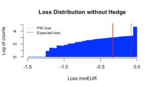
Our methodology allows us to undertake comprehensive impact assessments of credit-hedging measures. These in turn allow for more precise risk-based analysis for our clients.
See how credit risk impacts in your PPAs. Get in touch with us and learn to structure optimal contracts for today’s renewable energy market.