

In this short primer, we show how you can protect your portfolio against merchant risk and apply best-in-class risk management techniques.
While merchant risk management has recently been labeled as the “new frontier in renewables”, there is little consensus as to its implementation. If you are unfamiliar with power purchase agreement, check out our guide on what is a PPA.
DEFINITION: WHAT IS MERCHANT RISK?
In non-subsidised markets, unhedged asset revenues depend on the market price at which production is sold at the exchange. The financial risk posed by the moves of exchange prices is generally referred to as merchant risk.
While exchange-traded power prices have always been volatile, state subsidies are until now used to buffer their impact on revenue.
Where such schemes are being phased out, it is now up to project owners to handle merchant risk. Far from being a side-task of lesser relevance, the ability to understand and control merchant risk can determine the success of project financing.
PPAs become a crucial risk management tool that can contract a fixed offtake price over a long period.
HOW MATERIAL IS MERCHANT RISK?
Entering into a long-term fixed-price PPA means committing an offtake price in the face of uncertain future market prices. The generally accepted measure of uncertainty is volatility.
It measures the typical width of annual price fluctuation in percentage terms. For most European power markets, volatility is in the 15-30% range, meaning potential value fluctuations on the same order of magnitude. Clearly, a prudent investment approach will require some of this risk to be mitigated – how can this be done?
HEDGING 101: STACK-AND-ROLL
With PPAs in the 10-15 year tenor range, but only a few years (typically #1-5) being tradeable in the market, traders have devised the so-called stack-and-roll hedging technique. Initially, the total volume of the PPA is “stacked up” in a hedge which covers the liquid years.
To give an example, a 10 year PPA long position of 10MW (in total an equivalent of 100MW of a single yearly contract) could e.g. be hedged by selling 50MW each in the first two tradeable years.
Just before delivery of the PPA starts, the initial first-year hedge would be “rolled” forward to the then second year, and the volume reduced to 40MW, as 10MW start to go to delivery, as shown in the below picture.
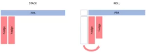
In doing so, the portfolio of PPA and hedge will always remain net zero volume. If prices for all tenors were to move strictly in parallel, this technique would ensure perfect hedging at all times. However, this is not the case – let’s delve into why …
WHY IS STACK-AND-ROLL NOT PERFECT ?
Most forward price curves feature time-dependent dynamic behavior. In the case of power, contracts with short time to maturity tend to be more volatile and less correlated to the long end of the power curve.

In other words, the simple stack-and-roll approach will not work perfectly. The reasons are as follows:
- Non-perfect correlation: Prices of the liquid front years will not move perfectly in line with the illiquid part of the curve. In other words, the value changes of the hedges will not perfectly offset the value changes of the illiquid parts of a PPA. The mismatch causes residual risk in the hedged PPA position.
- Volatility mismatch: The liquid hedges will be subject to higher volatility than the rest of the PPA, requiring an adjustment of hedging volumes. In particular, less volume of the more volatile hedges will be needed to balance out the risk of the less volatile longer-dated parts of the PPA.
We, therefore, have to acknowledge that perfect hedging is not possible. However, to get a better insight into exactly how big these residual risks are, we need to resort to slightly more involved simulation techniques.
GETTING PRICE DYNAMICS RIGHT
A suitable model choice for the power forward curve needs to account both for short- and long-term price dynamics. Two-factor models such as e.g. described in [Kiesel] are candidates for reflecting these properties. These models have the following distinctive features:
- Short end: The short end of the curve is subject to higher volatility than the rest of the curve. There is a time constant describing how far the “short end” of the curve reaches.
- Long end: The long end of the curve moves at constant volatility and thus tends to be stiff, i.e. all years further out than the short end will be almost perfectly correlated
- Short end – long end correlation: The correlation between the short end and the long end can be specified.
In order to “fit” the model to reality, volatilities and correlations of traded calendar year products are observed on a set of historical data. An optimisation algorithm ensures a choice of model parameters consistent with observations.
THE POWER OF SIMULATION – DISSECTING RISK
Starting from our initial considerations on merchant risk mitigation, we have discovered that risks incurred under realistic market conditions are quite complex.
Using Pexapark’s simulation engine, final sales revenue can be broken down into revenues, costs and all applicable risk adjustments. How all of these contributions stack up to final sales revenues can best be visualised in a waterfall chart:
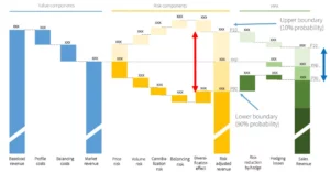
As indicated by the colours, there are three types of contributions to final sales revenue:
Value components:
- Expected baseload revenue: Sales revenues which would be achieved if production were (hypothetically) of baseload profile
- Expected profile markups/discounts: The technology- and geography-based price markup or discount of an asset due to its specific profile.
- Expected balancing cost: The cost of balancing due to forecasting errors
Risk components:
The risk components are pricing adjustments that accommodate for various non-hedgeable risks
- Price risk: The residual risk after hedging a position via stack-and-roll
- Volume risk: The revenue risk due to produced volumes differing from expected values
- Cannibalisation risk: Revenue risk due to price capture factors dropping more strongly than anticipated
- Balancing risk: The P90-adjustment to expected balancing costs
- Diversification effect: The (positive) P90-adjustment that reflects the diversification benefit from non-perfect correlation of the various sources of risk
PPA components:
- Cost of hedging: The discount that an offtaker charges the seller for assuming risk under a PPA deal
- Risk reduction: The positive P90 contribution that reflects the risk reduction of hedging an asset with a PPA
Note that all adjustment terms refer to the 90th percentile, i.e.they are downward adjustments. This is due to the fact, that pricing is done from an offtaker’s perspective, i.e. risk-adjustment means lowering the purchase price.
The positive adjustment terms shown in the waterfall graph are adjustments to referring to the 10th percentile. The range covered between P90 and P10 adjustments corresponds to the interval within which revenues materialise in 80% of all cases.
BENEFITS FOR RISK MANAGEMENT
The ability to dissect overall risk into all constituent sources of risk brings substantially more sophistication to the investment process: To name only a few topics, where simulation can add value:
- Investment decision & Structuring Process: Profit-at-Risk simulations of the PPA deal and its hedges allow for quantification of loss potential for any required confidence level.
- Hedging: The impact of hedging strategies on risk can be analysed, both with a view to Value-at-Risk (VaR) and Profit-at-Risk (PaR). Hedges can be defined arbitrarily, as a profile or as standard products. Risk can thus be assessed both from the perspective of a trader who stack-and-rolls, or from that of a corporate purchaser who is short and hedges with a PPA without stack-and-roll.
- Potential Future Exposures: Walk-forward simulations of the portfolio allow for measuring the potential future extent of replacement risk, both on the PPA deal and its hedges.
- Cashflows: Financial hedging of OTC deals may create a significant strain on cashflows. This can be readily quantified in a simulation framework.
- Stress-testing: By calibrating the simulation engine to different historical time windows, it is possible to assess portfolio dynamics for a range of market scenarios.
How are you protecting your portfolio against merchant risk? Get in touch with us today if you’d like to ask questions or to see how we use our simulation technique in the renewable investment process.